Principal Component Analysis (PCA) is a statistical method extensively used for dimensionality reduction in the field of machine learning and data science. The method essentially transforms a large set of variables into a smaller one that still contains most of the information in the larger set. In this article, we will explore how to apply PCA on a dataset using Python, with a focus on correlating parameters to a specific target.
Firstly, the necessary libraries are imported:
These libraries provide the required functionality for data manipulation, visualization and implementing PCA.
Next, the data is read from a CSV file: (You should prepare your dataset as csv;
Please consider your you delimiter is ; or ,
Delimitier is ; for my dataset
Subsequently, a specific column, Your_referance_Header', is set aside and all the columns that start with 'Parameter_Headers_Startswith_Shouldbe_Ignored' are dropped. The 'Your_referance_Header' column is then re-added to the DataFrame.
The correlation between 'Your_referance_Header' and other columns is computed:
The number of PCA components to be considered is then obtained from the user:
A for loop is initiated over the range of n_components, where PCA is applied to the top n_comp correlated parameters, and the explained variance is calculated for each n_comp.
A plot of the first principal component versus 'Your_referance_Header' is created:
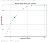
After looping over all the n_components, another plot of the explained variance ratio versus the number of PCA components is created. This assists in determining how many components are needed to explain a satisfactory amount of variance in the data:
The optimal number of PCA components is then determined:
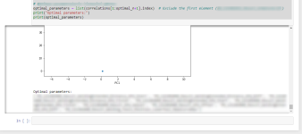
Finally, PCA is reapplied with the optimal number of components, and the resulting plot is displayed.
In the context of this script, the user is trying to find the most significant factors that correlate with the 'Reference_Column_Name'. By applying PCA, the user is able to reduce a large set of parameters to a more manageable number of 'principal components', which retain the most correlated information. This approach is particularly useful in scenarios where there are a large number of correlated variables.
Remember, before implementing PCA, it's crucial to standardize the features because PCA is a variance maximizing exercise. It projects your original data onto directions which maximize the variance.
In conclusion, PCA is a powerful tool for data analysis, visualization, and pre-processing for predictive modeling. It is essential in the toolkit of every data scientist or machine learning engineer.
Final codes are below:
Code first ask you for estimated PCA feature quantitiy. Please start from 2 and increase as much as goes. If you start with 200 parameter must probably you will get error. It works as below:


Also it gives you you optimal parameters headers as below and then you can build up your regression or Neural Network model with chosen optimum parameter:

Please write to me for re adjustment of your dataset.
Python Code Breakdown
Let's dive into the given code which represents a typical workflow for a PCA process:Firstly, the necessary libraries are imported:
Code:
import numpy as np
import pandas as pd
import seaborn as sns
import matplotlib.pyplot as plt
from sklearn.decomposition import PCA
from sklearn.preprocessing import StandardScaler
These libraries provide the required functionality for data manipulation, visualization and implementing PCA.
Next, the data is read from a CSV file: (You should prepare your dataset as csv;
Please consider your you delimiter is ; or ,
Delimitier is ; for my dataset
Code:
df = pd.read_csv('dataset_name.csv', delimiter=';')Subsequently, a specific column, Your_referance_Header', is set aside and all the columns that start with 'Parameter_Headers_Startswith_Shouldbe_Ignored' are dropped. The 'Your_referance_Header' column is then re-added to the DataFrame.
The correlation between 'Your_referance_Header' and other columns is computed:
Code:
correlations = df.corrwith(df['Your_referance_Header']).sort_values(ascending=False)The number of PCA components to be considered is then obtained from the user:
Code:
n = int(input("Enter the maximum number of PCA components to consider: "))A for loop is initiated over the range of n_components, where PCA is applied to the top n_comp correlated parameters, and the explained variance is calculated for each n_comp.
A plot of the first principal component versus 'Your_referance_Header' is created:
Code:
sns.scatterplot(x=f'PC1', y='Y', data=pca_df)After looping over all the n_components, another plot of the explained variance ratio versus the number of PCA components is created. This assists in determining how many components are needed to explain a satisfactory amount of variance in the data:
Code:
plt.plot(n_components, explained_variance, marker='o')The optimal number of PCA components is then determined:
Code:
optimal_n = np.argmax(explained_variance) + 1Finally, PCA is reapplied with the optimal number of components, and the resulting plot is displayed.
Importance and Application
The power of PCA lies in its ability to reduce the dimensional of a dataset while preserving its underlying structure. In other words, it transforms the data into a smaller dimension that captures the most important information. This reduction can drastically decrease the computational time for machine learning models and still maintain acceptable performance.In the context of this script, the user is trying to find the most significant factors that correlate with the 'Reference_Column_Name'. By applying PCA, the user is able to reduce a large set of parameters to a more manageable number of 'principal components', which retain the most correlated information. This approach is particularly useful in scenarios where there are a large number of correlated variables.
Remember, before implementing PCA, it's crucial to standardize the features because PCA is a variance maximizing exercise. It projects your original data onto directions which maximize the variance.
In conclusion, PCA is a powerful tool for data analysis, visualization, and pre-processing for predictive modeling. It is essential in the toolkit of every data scientist or machine learning engineer.
Final codes are below:
Code:
import numpy as np
import pandas as pd
import seaborn as sns
import matplotlib.pyplot as plt
from sklearn.decomposition import PCA
from sklearn.preprocessing import StandardScaler

# Read the dataset
df = pd.read_csv('your_data_set.csv', delimiter=';')

# Save 'Your_referance_Header' column to a separate variable
your_referance_header = df['Your_referance_Header']

# Remove columns that start with 'Parameter_Headers_Startswith_Shouldbe_Ignored'
df = df[df.columns.drop(list(df.filter(regex='^Parameter_Headers_Startswith_Shouldbe_Ignored')))]

# Re-add 'Your_referance_Header' column
df['Your_referance_Header'] = your_referance_header

# Calculate the correlation between 'Your_referance_Header' and all other columns
correlations = df.corrwith(df['Your_referance_Header']).sort_values(ascending=False)

# Get n value from the user
n = int(input("Enter the maximum number of PCA components to consider: "))

# Create n_components values for PCA
n_components = range(1, n + 1)
explained_variance = []

# Calculate PCA and explained variance values
for n_comp in n_components:
    # Determine parameters with highest n_comp correlation value
    top_n_columns = correlations[1:n_comp+1].index  # Exclude the first element (Your_referance_Header)

    pca = PCA(n_components=n_comp)
    df_scaled = StandardScaler().fit_transform(df[top_n_columns])
    pca_result = pca.fit_transform(df_scaled)
    explained_variance.append(sum(pca.explained_variance_ratio_))

    # Convert PCA result into a data frame
    pca_df = pd.DataFrame(data=pca_result, columns=[f'PC{i+1}' for i in range(n_comp)])

    # Add Your_referance_Header values
    pca_df['Y'] = your_referance_header

    # Plot PCA result
    plt.figure(figsize=(10, 8))
    sns.scatterplot(x=f'PC1', y='Y', data=pca_df)
    plt.title(f'PCA on Top {n_comp} Correlated Parameters')
    plt.show()

# Plot the explained variance ratio
plt.figure(figsize=(10, 8))
plt.plot(n_components, explained_variance, marker='o')
plt.xlabel('Number of PCA Components')
plt.ylabel('Explained Variance Ratio')
plt.title('Explained Variance Ratio for PCA Components')
plt.grid(True)
plt.show()

# Determine optimal number of PCA parameters
optimal_n = np.argmax(explained_variance) + 1
print("Optimal number of PCA components:", optimal_n)

# Apply PCA with optimal parameters
pca = PCA(n_components=optimal_n)
df_scaled = StandardScaler().fit_transform(df[top_n_columns])
pca_result = pca.fit_transform(df_scaled)

# Convert PCA result into a data frame
pca_df = pd.DataFrame(data=pca_result, columns=[f'PC{i+1}' for i in range(optimal_n)])

# Add Your_referance_Header values
pca_df['Y'] = your_referance_header

# Plot PCA result
plt.figure(figsize=(10, 8))
sns.scatterplot(x=f'PC1', y='Y', data=pca_df)
plt.title(f'PCA on Top {optimal_n} Correlated Parameters')
plt.show()

# Show the list of optimal parameters
optimal_parameters = list(correlations[1:optimal_n+1].index)  # Exclude the first element (Your_referance_Header)
print("Optimal parameters:")
print(optimal_parameters)
Code first ask you for estimated PCA feature quantitiy. Please start from 2 and increase as much as goes. If you start with 200 parameter must probably you will get error. It works as below:
Also it gives you you optimal parameters headers as below and then you can build up your regression or Neural Network model with chosen optimum parameter:
Please write to me for re adjustment of your dataset.
Attachments

Last edited: